Hull-White Interest Rate Model: Calibration, Pricing and Python Implementation Explained
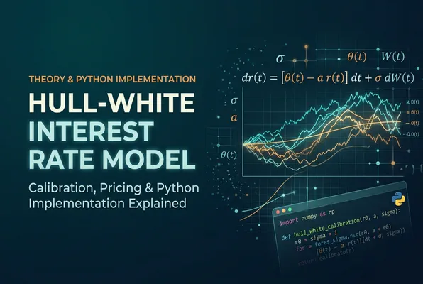

The Hull-White Interest Model is one of the most widely used short-rate models in quantitative finance. Introduced by John Hull and Alan White in 1990, it extends the classic Vasicek model so that it can fit today’s yield curve perfectly while still offering closed-form formulas for bonds and many popular interest rate derivatives. Banks, asset managers, insurers and risk teams rely on it for pricing, hedging and scenario generation.
This guide explains how the Hull-White Interest Model works, walks through its key equations in plain language, shows how to calibrate and simulate it, and discusses where it shines and where it falls short.
What Is the Hull-White Interest Model?
The Hull-White Interest Model is a one-factor, no-arbitrage, mean-reverting short-rate model. It describes how the instantaneous short rate r(t), the interest rate for an infinitesimally short period, evolves randomly over time. From the dynamics of that single rate, you can derive the entire term structure of interest rates, the prices of zero-coupon bonds and the values of options on those bonds.
Three properties make the model popular:
- Mean reversion: interest rates are pulled back toward a long-term level instead of drifting off indefinitely.
- Exact fit to the initial curve: the model reproduces today’s market discount factors by construction.
- Analytical tractability: bond prices, caps, floors and European swaptions have closed-form or near-closed-form solutions.
Because the short rate is normally distributed, the Hull-White Interest Model belongs to the family of Gaussian affine term structure models, which makes both calculation and implementation relatively straightforward.
The Hull-White Model Equation Explained
The most common form of the model is the one-factor Hull-White (also called the extended Vasicek) model. Under the risk-neutral measure, the short rate follows:
dr(t) = [θ(t) − a·r(t)] dt + σ dW(t)
Each term has a clear financial meaning.
Mean-Reversion Speed (a)
The parameter a controls how quickly the short rate is pulled back toward its mean. A large value of a means shocks fade quickly, while a small value means rate deviations persist for years. Mean reversion also determines how volatility is distributed across maturities: higher a reduces the volatility of long-term rates relative to short-term rates.
Volatility (σ)
The parameter σ is the volatility of the short rate. In the basic version of the model it is constant, though extended versions allow it to be time-dependent to fit a full set of option prices. Higher σ widens the distribution of future rates and raises option values.
The Time-Dependent Drift θ(t)
The function θ(t) is what separates the Hull-White Interest Model from Vasicek. It is chosen so that the model matches the observed forward curve:
θ(t) = ∂f(0,t)/∂t + a·f(0,t) + (σ²/2a)·(1 − e^(−2at))
Here f(0,t) is the instantaneous forward rate observed in the market today. Intuitively, θ(t) tells the model where rates are expected to go, based on what the market curve already implies, while the −a·r(t) term pulls the simulated rate back toward that path.
Wiener Process W(t)
The term dW(t) is the increment of a Brownian motion, the source of randomness. Because it is Gaussian, the short rate at any future time is normally distributed, with a mean and variance that can be written down explicitly.
The Mathematical Foundation of the Hull-White Model
Todefine Hull White more precisely, it is useful to examine its mathematical structure and its derivation from the broader class of no-arbitrage models. The Hull White model is a flexible model for interest rate modeling in which the drift component is time dependent and can be adjusted to reflect changing market expectations. This feature allows practitioners to relate theoretical interest rate movements to observable market data. A key assumption is that the short rate follows a normal distribution, meaning that future interest rate values can be positive or negative. Under this framework, the model provides a consistent way to calculate future discount factors and zero coupon bond prices while maintaining compatibility with the initial market environment.
Hull-White vs. Vasicek, CIR and Other Short-Rate Models
Choosing a model starts with understanding how it compares with the alternatives.
| Feature | Vasicek | CIR | Ho-Lee | Hull-White | Black-Karasinski |
|---|---|---|---|---|---|
| Mean reversion | Yes | Yes | No | Yes | Yes |
| Fits initial yield curve | No | No | Yes | Yes | Yes |
| Negative rates possible | Yes | No | Yes | Yes | No |
| Closed-form bond prices | Yes | Yes | Yes | Yes | No |
| Distribution of r | Normal | Non-central chi-square | Normal | Normal | Lognormal |
Compared with Vasicek, Hull-White adds the time-dependent θ(t) to match the market curve. Compared with Ho-Lee, it adds mean reversion, which gives a more realistic volatility term structure. Compared with CIR, it permits negative rates, an increasingly valuable property in modern markets. Compared with Black-Karasinski, it trades the lognormal rate distribution for far greater analytical convenience.
Bond Pricing Under the Hull-White Interest Model
One of the biggest strengths of the Hull-White Interest Model is its affine bond pricing formula. The price at time t of a zero-coupon bond maturing at T is:
P(t,T) = A(t,T) · exp(−B(t,T) · r(t))
where
B(t,T) = (1 − e^(−a(T−t))) / a
and A(t,T) is a function built from today’s discount curve, σ and a. Because of this structure:
- Bond prices are exponential-affine in the short rate.
- Yields are linear in r(t), which makes the model easy to use for hedging and sensitivity analysis.
- The model reproduces the initial discount curve exactly, so P(0,T) equals the market price for every maturity.
This is a major advantage over models that need an approximate fit to the yield curve.
Pricing Caps, Floors and Swaptions
Since bond prices are lognormal under the T-forward measure in the Hull-White framework, European options on zero-coupon bonds have a Black-Scholes-style closed-form solution. This is the foundation for pricing other products.
Caps and Floors
A cap is a portfolio of caplets, and each caplet can be expressed as a put option on a zero-coupon bond. Using the bond option formula, a full cap or floor can be priced analytically, which makes caps and floors the natural instruments for calibrating a and σ.
European Swaptions
European swaptions can be priced using Jamshidian’s decomposition, which converts an option on a coupon bond into a sum of options on zero-coupon bonds. This requires solving for a critical short rate r* with a one-dimensional root search, after which the price is a simple sum of closed-form terms. The result is a fast and accurate swaption pricer.
Bermudan and Callable Products
For Bermudan swaptions, callable bonds and other path-dependent or early-exercise instruments, no closed-form solution exists. In these cases the model is implemented using:
- Trinomial trees (the original Hull-White tree construction)
- Finite difference methods for the pricing PDE
- Monte Carlo simulation with regression methods such as Longstaff-Schwartz
The Hull-White tree is especially popular because it is built to match the initial yield curve and is simple to extend to American-style features.
Numeraire Choice and Financial Applications
Another important aspect of Hull-White is the relationship between interest rate modeling and the concept of a numeraire. In risk-neutral valuation, the selected numeraire determines the probability measure under which discounted asset prices behave as martingales. For example, when pricing a zero coupon bond option, the corresponding bond can serve as the numeraire, simplifying the valuation process. The holder of a financial contract is then exposed to changes in the underlying interest rate, which influence the contract’s market value and potential payoff. In this context, the parameter k may represent a strike rate or another contract-specific input, depending on the instrument being valued. Understanding these relationships helps explain how the Hull-White framework connects mathematical assumptions with practical derivative pricing.
How to Calibrate the Hull-White Interest Model
Calibration is where theory meets market data. The goal is to select a, σ and θ(t) so the model is consistent with observable prices.
Step 1: Fit θ(t) to the Yield Curve
Start by building a discount curve from market instruments such as deposits, futures, FRAs and swaps (and, in the post-LIBOR world, overnight risk-free rate swaps). Then derive the instantaneous forward curve f(0,t) and compute θ(t). In practice this is done implicitly: the model is constructed so that P(0,T) equals the market discount factor for all maturities.
Step 2: Calibrate a and σ to Option Prices
With θ(t) fixed, the remaining parameters are fitted to liquid volatility instruments:
- Choose a calibration set, typically at-the-money caps or a co-terminal or diagonal set of European swaptions that matches the product you want to price.
- Compute model prices using the analytical formulas.
- Minimize the sum of squared differences between model and market prices (or implied volatilities), for example with Levenberg-Marquardt or another least-squares optimizer.
Parameter Estimation and Model Conditions
In practical applications, financial analysts must carefully calibrate parameters to ensure that the model produces realistic results. This process involves selecting appropriate values for the mean-reversion coefficient and volatility, while considering the market conditions under which the model is applied. A model like Hull-White can also be extended by introducing additional restrictions or a specific optimization condition to improve its performance for particular financial instruments. For example, a calibration procedure may aim to minimize pricing errors while respecting a predefined maximum deviation from observed market prices. The choice of calibration instruments and numerical methods is therefore important for obtaining stable and economically meaningful results.
Practical Calibration Tips
- Match the instruments to the product. To price a 10-year Bermudan swaption, calibrate to the swaptions that correspond to its exercise dates and final maturity.
- Beware of a and σ instability. Mean reversion is notoriously hard to pin down. Some practitioners fix a from historical or expert judgment and calibrate only σ.
- Use piecewise-constant σ(t). Allowing volatility to vary by period lets the model fit a whole strip of swaptions or caplets exactly.
- Check parameter stability over time. Large day-to-day jumps in calibrated values are a warning sign.
Simulating the Hull-White Interest Model
Monte Carlo simulation is essential for risk management, XVA, ALM and any product without an analytical price.
Exact Discretization
Because the short rate is Gaussian, it can be simulated exactly, without discretization error. A common approach is to write r(t) = x(t) + α(t), where x(t) follows a zero-mean Ornstein-Uhlenbeck process and α(t) is a deterministic function that absorbs the initial curve:
x(t+Δ) = x(t)·e^(−aΔ) + σ·√((1 − e^(−2aΔ)) / 2a) · Z
with Z a standard normal draw. The deterministic shift α(t) is then added back to recover r(t) on each path.
Simulation Workflow
- Calibrate a, σ and fit the initial curve.
- Generate normal random numbers (use antithetic variates or Sobol sequences to reduce variance).
- Evolve x(t) over the time grid.
- Compute the short rate, discount factors and, if needed, full forward curves on each path and date.
- Value the instrument or portfolio and average across paths.
Because the bond pricing formula is analytic, you can reconstruct the entire yield curve at every simulation node from the single state variable, which is extremely convenient for exposure calculations.
Real-World Applications of the Hull-White Interest Model
Derivative Pricing and Hedging
Trading desks use the model for vanilla and exotic interest rate derivatives, including Bermudan swaptions, callable and putable bonds, and range accruals.
Counterparty Credit Risk and XVA
Interest rate scenarios drive the exposure profile of swaps and other derivatives. Hull-White is a standard choice for simulating rates when computing CVA, DVA and FVA, thanks to its speed and exact curve fit.
Asset-Liability Management
Insurers and pension funds use Hull-White scenarios to project liabilities and assets under many rate paths, supporting economic capital and solvency analysis.
Regulatory Stress Testing and Economic Scenario Generation
Gaussian short-rate models provide a transparent, controllable way to generate yield curve scenarios, including negative rate regimes.
Mortgage and Prepayment Modeling
The simulated rate paths feed prepayment and option-adjusted spread (OAS) analyses for mortgage-backed securities.
Strengths of the Hull-White Interest Model
- Perfect fit to today’s yield curve through θ(t)
- Analytical tractability for bonds, caps, floors and European swaptions
- Realistic mean reversion and a sensible volatility term structure
- Fast calibration to liquid instruments
- Exact simulation with no discretization bias
- Ability to handle negative interest rates
- Flexible numerical implementation via trees, PDEs and Monte Carlo
Limitations and Criticisms
No model is perfect, and understanding the weaknesses of the Hull-White Interest Model is essential for using it responsibly.
- Single factor: all rates across the curve are perfectly correlated, so the model cannot generate independent moves in short and long rates, such as curve twists, steepening or flattening not tied to the level factor. Two-factor extensions (G2++ or Hull-White two-factor) address this.
- No volatility smile: the basic model has normal (Gaussian) dynamics and does not reproduce skew or smile in cap and swaption volatilities. For smile-sensitive products, consider SABR, LMM with stochastic volatility or shifted/displaced alternatives.
- Parameter instability: calibrated mean reversion can be unstable, and results for exotic products can be sensitive to this choice.
- Short-rate focus: the model is specified on an unobservable instantaneous rate, whereas market practice often prefers modeling observable forward or swap rates, as in the LIBOR/forward market model.
- Normal rates: the Gaussian assumption means rates can reach implausibly large positive or negative values in the tails, particularly over long horizons.
Extensions of the Hull-White Model
Over the years, several extensions have broadened the model’s usefulness:
- Two-factor Hull-White / G2++: adds a second, correlated factor to create richer curve dynamics and decorrelate short and long rates.
- Time-dependent volatility σ(t) and mean reversion a(t): improves fit to the term structure of volatilities.
- Multi-curve frameworks: separate discounting (OIS) and projection curves, which became the market standard after the financial crisis.
- Cross-currency and inflation versions: Hull-White is used as the building block for FX hybrid models and Jarrow-Yildirim-type inflation models.
- Hull-White with stochastic volatility: introduces a volatility process to better capture smile effects.
Implementing the Hull-White Interest Model in Practice
Whether you code the model yourself or use a library, a few practical guidelines help avoid common pitfalls.
Choosing Tools
Popular open-source options include QuantLib (C++ with Python bindings), which has built-in Hull-White processes, tree engines and calibration helpers. In Python, you can also implement the model directly with NumPy: the exact simulation scheme is only a few lines of code.
Best Practices
- Build a clean curve first. Errors in the discount curve propagate directly into θ(t) and every price.
- Select calibration instruments deliberately, aligned with the risk you want to capture.
- Validate by repricing the calibration instruments and checking that the model reproduces them within tolerance.
- Test sensitivity to the mean-reversion parameter and compare against alternative models for exotic products.
- Monitor parameter drift and recalibrate regularly.
A Simple Conceptual Example
Suppose the 10-year zero rate is 3% and you want to price a 5-year European payer swaption on a 5-year swap. You would:
- Build the discount curve and derive f(0,t).
- Calibrate a and σ to a set of 5y-into-5y and nearby swaptions.
- Use Jamshidian’s decomposition to compute the swaption price from closed-form bond put prices.
- Cross-check by Monte Carlo using the exact simulation scheme.
If the analytical and simulated prices agree, you have a reliable valuation engine.
When Should You Use the Hull-White Interest Model?
The Hull-White Interest Model is an excellent choice when:
- You need an exact fit to the current yield curve.
- Speed and tractability matter, for example in XVA or large-scale scenario generation.
- You are valuing Bermudan swaptions or callable bonds where a robust, well-understood lattice or PDE approach is helpful.
- Moderate accuracy for the volatility surface is acceptable, and smile effects are secondary.
Consider alternatives when smile or skew matters (SABR, stochastic-volatility LMM), when you need independent curve movements (multi-factor models), or when you must model the full forward curve directly (Heath-Jarrow-Morton, LIBOR market model).
Conclusion
The Hull-White Interest Model remains a cornerstone of interest rate modeling because it strikes a rare balance: it matches the market yield curve exactly, captures mean reversion, supports negative rates and offers analytical formulas for the most important building-block instruments. Its limitations, particularly the single-factor structure and lack of smile, are well understood, and a rich family of extensions exists to address them.
Whether you are pricing a swaption, simulating thousands of rate scenarios for credit exposure or exploring how interest rate risk affects a long-term portfolio, understanding the Hull-White Interest Model gives you a dependable, transparent framework. Master its calibration, know its boundaries, and it will serve as a reliable workhorse in your quantitative toolkit.
For more practical guides on financial modeling, risk and quantitative methods, explore the resources at finflexia.app .

Written by
Dominik KonoldFounder
Dominik is the founder of Finflexia and an expert in treasury accounting, financial instrument valuation and IFRS compliance. Since 2016, he's been a certified Professional Risk Manager (PRMIA) and also lectures for the Association of Public Banks and the Academy of International Accounting. He built Finflexia to help treasury teams automate complex accounting workflows.
Related Posts
Interest Rate Floor Explained
This Guide provides an overview of interest rate caps and floors in lending, explaining how they set upper and lower limits on variable interest rates in loan contracts and protect lenders and borrowers from extreme market movements.

What Is an Interest Rate Swap?
This guide explains interest rate swaps, including how they work, their types, valuation, benefits, risks, and role in managing interest rate risk.

What Is an FX Swap? Understanding Foreign Exchange Swaps
This article explains what an FX swap is, how it works, and how it is used to manage foreign currency, liquidity, and financial risks.
Ready to simplify your treasury accounting?
See how Finflexia helps you manage financial instruments with ease. Book a demo to learn more.
Book a Demo